How to change raster appearance?

Apart from using vectors (like points, lines, and polygons) on your maps, in GIS Cloud you can also add and use raster images (for example satellite or drone imagery, vegetation indices, etc.). Before uploading data, first, make sure to check which spatial raster files are supported. GIS Cloud currently supports multiband and single-band raster types. Multiband is the default render setting, and the Single-band setting can be used with both single-band and multiband files (for example, select just one band to use for classification).

GIS Cloud supports these raster file types: .tif, .tiff, .jpg, .png, .gif, .img, .sid, .jp2

If the raster is not georeferenced, don’t forget to upload the projection file too. If the raster doesn’t have the projection file, it won’t fit the map.

If you’re also looking for how to upload your rasters, or how to add a raster mosaic, check out the following guides: How to add rasters to the map?, How to add raster mosaic?

Working with single-band rasters

Once you’ve uploaded your raster to GIS Cloud, you can add the file as a new layer to your map by choosing Add layer, and selecting the relevant file from the File Manager or your external database in Database Manager. For single-band rasters, you must first choose the visualisation method before you can see the layer on the map! You can access the style settings by opening the Layer properties (double-click on the layer).

When using a single-band raster file, the system will automatically recognize that the added raster is single-band, and will set the Render type accordingly. It is not possible to switch the render type to Multiband since the file only contains one band.

If you’re working with a single-band raster, the Classification Wizard will automatically open for you to modify the appearance settings. You can classify raster files based on the pixel values by choosing different rendering methods, ranges, and number of classes. Classifying rasters is useful for creating thematic maps, for example showing different land use or land cover classes, or to visualise different vegetation indices.

If you prefer a video tutorial, check out our walkthrough at the end!

Using the ‘Classified’ rendering method

The ‘Classified’ rendering method considers the distribution of values and groups the values into the number of breaks or colors you want to display. A color map is useful when you want to select a color for each pixel value.

Follow the steps below to classify a single-band raster:

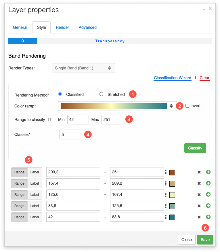
1. Select the Classified rendering method – this rendering method assigns a color for each class or group of values.
2. Choose your color ramp (you can also choose to invert the colors, for example if the ramp is black-white, you can invert it to white-black).
3. Define the range by entering the minimum and maximum pixel values. Anything outside of that range will not be shown on the render.
4. Define the number of classes you wish to create and click on Classify.
5. You can manually adjust the range that was selected automatically and the label for each class separately, as well as adjust colors. Note that the values should not overlap.
6. Save your work and take a look at your raster layer on the map!

Note: If you’re working with a multiband file but have selected to classify it as a single-band, you will also be able to choose which band you wish to use for classification.

Using the ‘Stretch’ rendering method

Similarly to the classified method, ‘Stretched’ will allow you to assign colours to pixel values, but instead of a separate fixed number of classes, it takes the range of all values in your data and stretches it to fit within a data type range. In practice, this means that your layer will be visualised as a gradient of your color ramp, as opposed to the separate classes with the other method.

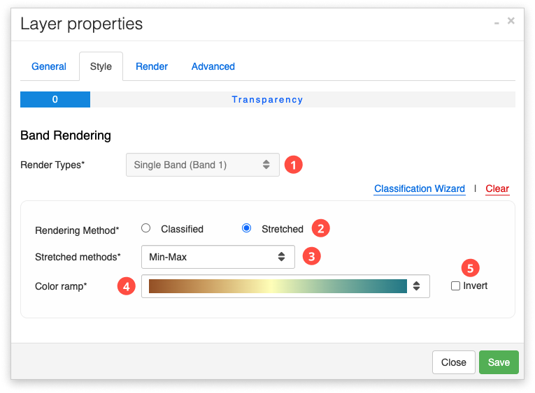
Follow the steps below to classify a single-band raster:

1. Select the render type (single-band)
2. Select the Stretched rendering method.
3. Choose between one of the stretch methods available:
   • None – No stretch method is applied to the layer, even if statistics exist.
   • Min-Max – Applies a linear stretch based on the output minimum and output maximum pixel values, which are used as the endpoints for the histogram. For example, in an 8-bit dataset, the minimum and maximum values can be 33 and 206. A linear stretch is used to distribute the values across 256 values, from 0 to 255. This increases the ability to see differences in values throughout the dataset. Minimum Maximum is a good choice for standardizing the appearance of multiple rasters for comparison.
   • Percent clip – Cuts off a percentage of the highest and lowest values and applies a linear stretch to the remaining values across the available dynamic range of the data type. This reduces the effects of outliers and enhances the remaining data. You can specify the percentage of the low and high values to exclude from the stretch. Valid values range from 0 to 99.
   • Histogram equalization – Applies the specified piecewise histogram to display the pixels values. The piecewise histogram allows you to map the input pixel values to a rendered value.
   • Standard deviation – Applies a linear stretch between the values defined by the standard deviation (n) value. For example, if you define a standard deviation of 2, the values beyond the second standard deviation become 0 or 255, and the remaining values are linearly stretched between 0 and 255. You can specify the n value for the number of standard deviations to use. This method is used to emphasize how much feature values vary from the mean value; it is best when used on normally distributed data.
4. Choose your color ramp
5. You can also choose to invert the colors, for example if the ramp is black-white, you can invert it to white-black.
6. Save your work and take a look at your raster layer on the map!

Working with multiband rasters

Multiband rasters are rasters that contain more than one band. Multiband is the default render types for multiband rasters, but they can also be used with the single-band render type if you want to use just one of the available bands for classification.

There are no additional steps required when working with multiband rasters, but you can still use the Render options for further adjustments.

Render options

Raster interpolation

Changing the raster interpolation method works for single-band and multiband rasters. Resampling is the process of interpolating the pixel values while transforming your raster dataset.

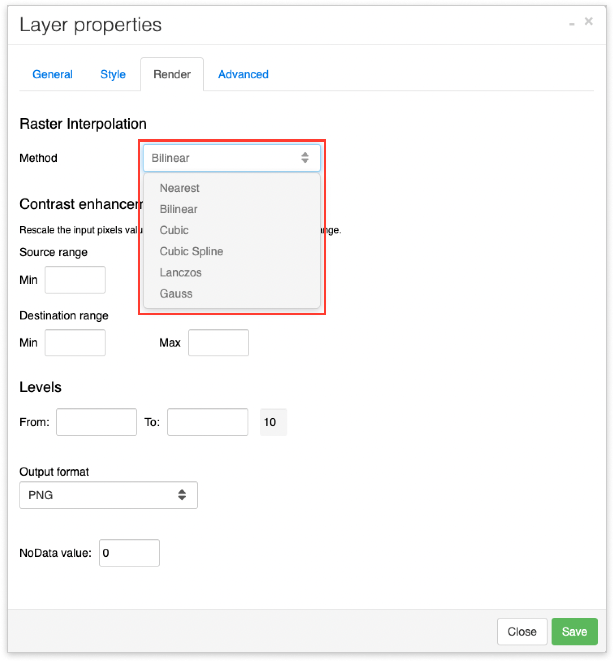
In GIS Cloud you can choose between 5 different interpolation methods from the drop down menu.

• Nearest – This is the default method. Performs a nearest neighbour assignment and is the fastest of the interpolation methods. It is used primarily for discrete data, such as a land-use classification, since it will not change the values of the cells.
• Bilinear – Performs a bilinear interpolation and determines the new value of a cell based on a weighted distance average of the four nearest input cell centres. It is useful for continuous data and will cause some smoothing of the data.
• Cubic – Performs a cubic convolution and determines the new value of a cell based on fitting a smooth curve through the 16 nearest input cell centres. It is appropriate for continuous data, although it may result in the output raster containing values outside the range of the input raster. Geometrically it is less distorted than the raster achieved by the nearest neighbour resampling algorithm.
• Cubic spline – an interpolation method in which cell values are estimated using a mathematical function that minimises overall surface curvature, resulting in a smooth surface that passes exactly through the input points.
• Lanczos – an interpolation method used to compute new values for sampled data. It is often used in multivariate interpolation, for example for image scaling (to resize digital images), but can be used for any other digital signal.
• Gauss – applies a Gaussian convolution to the source raster and calculates pixel value using the distance-weighted value of four nearest pixels from the blurred raster.

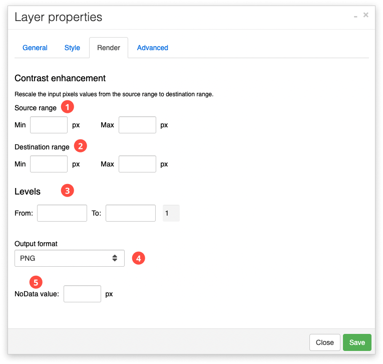
Other render options

(1) and (2) One of the functions is to rescale the input pixels from the source range to the destination range. Since each raster has an input range of colors, the range has values between 0 and 255 where each value represents one color. It is possible to change the range of colors in the raster by changing the values in the destination range.

(3) If you want your raster to only appear on certain zoom levels, you can define the zoom level range here. The current zoom level is displayed on the right.

(4) Also, it is also possible to change the output format for the raster on the map. This option is usually used when the black edges in rasters are removed. To remove black edges, set the output format to PNG, then change the NoData value (5) to 0 (note: if the edge is white, use 255 instead).

Video Tutorial